NAEP Technical DocumentationTrimming the Nonresponse Adjusted Student Weights

Student weights that contributed too large a proportion to the overall variance were trimmed, which reduces the overall variance, at the potential cost of a slight bias (the overall mean square error should be reduced by this operation).

In the 2001 assessment, a new trimming algorithm for student weights was used. The old approach (used for school weights in 2001 as is discussed in School Trimming) was an iterative process in which the algorithm was executed multiple times until convergence was reached. The NAEP sampling and weighting contractor developed a new algorithm that is not iterative, but results in the same trimming adjustments as the old iterative approach. This new time-saving procedure will be used for future NAEP trimming operations now that the algorithm has been successfully executed for the 2001 geography and U.S. history assessment student weights.

The starting point is the summation of the nonresponse-adjusted student weights w_ij × STNR_k over all assessed and excluded students within each school i:

Define

The trimming criterion requires that the x_i should satisfy

where T = 10/n. This criterion can be interpreted as saying that no school should contribute more than the fixed proportion T to the overall variance at the school level of its nonresponse-adjusted student weights. If the initial summations x_i satisfy this condition as is, then there is no trimming, i.e., the trimming adjustments STUDTRIM_i are all set to 1.

Otherwise the new algorithm (as did the old algorithm) sorts the schools in descending order of . This order is maintained as the x_i values are altered, so the order can be viewed as fixed even as the x_i values alter. Thus i=1 corresponds to the largest , i=2 to the next largest, etc. (Note that these largest values exceeding the T value in practice always correspond to large x_i values, so for these large values this order corresponds to a descending order by x_i.) With this reordering, the values of i such that

will be i=1,…,c.

The idea behind the new algorithm is to look at the x_i values as they would be if the first e records on this listing are trimmed. The e trimmed values will all be equal to a fixed value x_d that satisfies

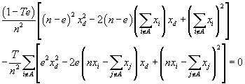
Although trimming factors may vary, the x_d will be invariant across all trimmed school records and the expression to the right of the equal sign may be rewritten as

where e is the number of records trimmed and A is the set of records trimmed. Gathering all terms to the left of the equal sign gives

which may be rewritten as

open paren 1 minus T times e closed paren times open bracket open bracket open paren n minus e closed paren times x sub d minus summation over i not an element of A of x sub i closed bracket divided by n closed bracket squared minus T times summation over i not an element of A open bracket open paren n times x sub i minus e times x sub d minus summation over j not an element of A of x sub j closed paren divided by n closed bracket squared equals 0

After the squared expressions are expanded this becomes

open bracket open paren 1 minus T times e closed paren divided by n squared closed bracket times open bracket open paren n minus e closed paren squared times x sub d squared minus 2 times open paren n minus e closed paren times open paren summation over i not an element of A of x sub i closed paren times x sub d plus open paren summation over i not an element of A of x sub i closed paren squared closed bracket minus open paren T divided by n squared closed paren times summation over i not an element of A open bracket e squared times x sub d squared minus 2 times e times open paren n times x sub i minus summation over j not an element of A of x sub j closed paren times x sub d plus open paren n times x sub i minus summation over j not an element of A of x sub j closed paren squared closed bracket equals 0

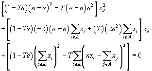
which can be rewritten as a quadratic equation in x_d

open bracket open paren 1 minus T times e closed paren times open paren n minus e closed paren squared minus T times open paren n minus e closed paren times e squared closed bracket times x sub d squared plus open bracket open paren 1 minus T times e closed paren times negative 2 times open paren n minus e closed paren times open paren summation over i not an element of A of x sub i closed paren plus 2 times T times e squared times summation over i not an element of A of x sub i closed bracket times x sub d plus open bracket open paren 1 minus T times e closed paren open paren summation over i not an element of A of x sub i closed paren squared minus T times summation over i not an element of A open paren n times x sub i minus summation over j not an element of A of x sub j closed paren squared closed bracket equals 0

This further simplifies to

open paren n minus e closed paren times open paren n minus e minus T times e times n closed paren times x squared sub d minus 2 times open paren n minus e minus T times e times n closed paren times open paren summation over i not an element of A of x sub i closed paren times x sub d minus T times n squared times summation over i not an element of A of x sub i squared plus open paren 1 plus T times n closed paren times open paren summation over i not an element of A of x sub i closed paren squared equals zero

Substituting 10/n for T in the above expression gives

Solving for x_d produces

where

is the mean of the x_i for untrimmed school records, and

sigma squared sub x prime, equals open bracket summation over i not an element of A of x squared sub i divided by open paren n minus e closed paren closed bracket minus open bracket summation over i not an element of A of x sub i divided by open paren n minus e closed paren closed bracket

is the variance of the x_i among untrimmed school records.

The critical problem that led to the use of an iterative process in the past is that after trimming e records and assigning a new x_d to these records the recomputed and sum of squares may indicate that further records (e.g., record e+1) may now violate the trimming criterion. Under the new procedure, an x_d is generated according to these formulas for each and every potential value of e, going down the sorted list in one single step. The correct final value of e is the first e value for which the recomputed x_i's, the sum of squares, and proportions of sum of squares all satisfy the trimming criterion.

This table shows the trimming factors computed for each grade and NAEP region. The smallest trimming factor was 0.700 in fourth grade, Southeast NAEP region. The largest number of trimmed schools was 6 in grade 8, West NAEP region.

Student weight trimming factors, by region and grade, national main assessment: 2001
Grade	Region	Non-unity trimming factors
4	Northeast	†
	Southeast	0.700	0.706	0.769	0.820	0.989
	Central	†
	West	0.944	0.953	0.987
8	Northeast	†
	Southeast	0.899	0.930	0.992
	Central	†
	West	0.794	0.845	0.858	0.887	0.926	0.927
12	Northeast	†
	Southeast	0.906	0.947
	Central	†
	West	0.838	0.937	0.992
† Not applicable; no trimming factors were applied for these NAEP regions. SOURCE: U.S. Department of Education, Institute of Education Sciences, National Center for Education Statistics, National Assessment of Educational Progress (NAEP), 2001.

These trimming factors are written as STUDTRIM_i for each school i (though they are assigned to the student weights they are equal within schools). Untrimmed schools receive STUDTRIM_i factors of 1.

The student weight at the end of the processes described is called the "pre-poststratification student weight," as it is the student weight preceding the final step of poststratification. This weight can be defined as

prew_ij = w_ij × STNR_k × STUDTRIM_i × HORG_ij

HORG_ij is the inverse of the probability the student was assigned a geography or U.S. history assessment (see Assigning Assessments as U.S. History and Geography). At this point in the process, the weights are specific to the subject-area assessment.

Last updated 26 August 2008 (FW)

Printer-friendly Version