- Surveys & Programs
- Data & Tools
- Fast Facts
- News & Events
- Publications & Products
- About Us
Table of Contents | Search Technical Documentation | References
NAEP Technical DocumentationComputation of Measures of Size
|
Setting Measures of Size for Each Jurisdiction in State NAEP 2003 |
|||
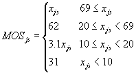
For the main school sample for State NAEP the initial measure of size MOSjs for school s in jurisdiction j is a function of xjs, the total number of students in school js in the respective grade (fourth or eighth):

Putting aside the very small schools (xjs less than 20), the measure of size (MOS) is constant for schools with smaller enrollment (up to 68), and proportional to xjs for schools with larger enrollment (69 and above), as outlined in the formulation for obtaining a self-weighting student sample. For the schools with xjs less than or equal to 10, the MOS is also constant, but half that of the “medium” schools (xjs from 20 to 68). The students in these schools are selected at half the rate of those in the medium schools, as desired. Schools with 10 to 20 students have a sliding factor of 1/2 to 1 in relative probabilities.
The probability of selection for each school is essentially this MOSjs multiplied by a constant of proportionality bj which is carefully calculated for each jurisdiction j and grade. The proportionality constant bj is computed to achieve the target of Tj equal to 6,510 as closely as possible, under a maximum burden constraint defined below.
Multiple hits are allowed for large schools. With Hjs as the random variable determining the number of hits (Hjs = 0, 1, 2, 3, . . .), schools for which Hjs is 0 are not included in the school sample. If Hjs ![]() 1, the school is sampled. The desired student sample size is then essentially 62 × Hjs (62 for one-hit schools, 124 for two-hit schools, etc.). There is, however, an added twist. The final student sample size for each sampled school is computed according to the following function:
1, the school is sampled. The desired student sample size is then essentially 62 × Hjs (62 for one-hit schools, 124 for two-hit schools, etc.). There is, however, an added twist. The final student sample size for each sampled school is computed according to the following function:

The A( ) function is the “almost all” function. When a school's target population xjs is only slightly larger than the desired sample size 62 × Hjs (by a factor of from 1 to 69/62), the sampling plan increases the sample size to equal the target population. This function avoids samples which exclude a handful of students in the grade, something that schools usually prefer to avoid. For example, a school with two sample hits (Hjs = 2) has a desired sample size of 124. If the school has anywhere up to 137 students, all students are taken. If the school has 138 or more students, the design calls for a sample of 124 students exactly.
The next step in the development is to characterize the sampling distribution of Hjs, which essentially defines the school and student sample design. Let Ejs = E(Hjs), the expected number of hits. Write [Ejs] as the integer part of Ejs; that is, the largest integer smaller than Ejs. Define ![]() as the probability of selection of the school into the sample (i.e.,
as the probability of selection of the school into the sample (i.e., ![]() equals the probability that Hjs
equals the probability that Hjs ![]() 1). The relationship among Hjs, Ejs, and
1). The relationship among Hjs, Ejs, and ![]() is as follows in all NAEP school samples:
is as follows in all NAEP school samples:
-
0 < Ejs < 1: Hjs equals 0 or 1,
 = Ejs.
 -
Ejs = n, n = 1, 2, … Hjs,
 = 1.
= 1. -
n < Ejs < n+1, n = 1, 2, . . . :
Hjs = n with probability 1 – {Ejs – [Ejs]}
Hjs = n+1 with probability Ejs – [Ejs]
Note that the sampling distribution of the random variable Hjs = n is now fully specified, once Ejs is defined for each school. The following formula defines Ejs:
![]()
The quantity uj (the maximum number of “hits” allowed) in this formula is designed to put an upper bound on the burden for the sampled schools. In most jurisdictions, uj was set to 3. In smaller jurisdictions, uj was set to a larger value to allow for a larger expected student sample size. The largest values of uj were
-
four for the Atlanta Trial Urban District Assessment district grade 8,
-
four for Wyoming grade 8,
-
five for Delaware grade 8, and
-
eight for Alaska grades 4 and 8.
The last task in this development is to delineate the computation of bj for each jurisdiction. This delineation is done in an iterative fashion. In the kth iteration, compute Ejs(k) values for each school based on an intermediate value of bj(k). This computation defines a distribution for Hjs, and thus for yjs. The overall expected yield of students is then
![]()
with Sj the set of schools in the jurisdiction j frame, and Ek indicating expectations using bj(k). The value Tj(k) is compared with the desired target Tj. If Tj(k) does not equal Tj (rounded to an integer), then the process continues to a k+1st iteration, computing bj(k+1) as some value in the interval [bj,bj(k)×Tj/Tj(k)], and continues iteratively until bj(k) satisfies
![]()
after rounding to integer values.
Last updated 02 October 2008 (KL)